16 Affine Transformations
We have been looking at change of basis in vector spaces, and I have described these as change of choice of coordinates. But some applications need to allow a broader class of choice of coordinates. In particular, any change of basis leaves the origin, $\vec 0$, unchanged, since any linear transformation maps the origin to the same point. If we also want to be able to move the origin of the coordinate system, we can use "affine transformations." To keep things simple, we will consider only affine transformations from $\R^n$ to itself. Note that this material is not from the textbook.
Definition: An affine transformation from $\R^n$ to $\R^n$ is a linear transformation (that is, a homomorphism) followed by a translation. Here a translation means a map of the form $T(\vec x) = \vec x + \vec c$ where $\vec c$ is some constant vector in $\R^n$. Note that $\vec c$ can be $\vec 0$, which means that linear transformations are considered to be affine transformations.
We are particularly interested in affine transformations that are bijections, but non-bijective affine maps are also possible.
Suppose $f\colon \R^n\to\R^n$ is an affine transformation. Then there is an $n\times n$ matrix, $A$, and a vector $\vec c\in\R^n$ such that $f(\vec x) = A\vec x + \vec c$. Written out in full this looks like $$ f\begin{pmatrix} x_1\\x_2\\ \vdots\\ x_n \end{pmatrix} = \begin{pmatrix} a_{11} & a_{12} & \cdots & a_{1n} \\ a_{21} & a_{22} & \cdots & a_{2n} \\ \vdots& \vdots & \ddots & \vdots \\ a_{n1} & a_{n2} & \cdots & a_{nn} \end{pmatrix} \begin{pmatrix} x_1\\x_2\\ \vdots\\ x_n \end{pmatrix} + \begin{pmatrix} c_1\\c_2\\ \vdots\\ c_n \end{pmatrix} = \begin{pmatrix} a_{11}x_1 + a_{12}x_2 + \cdots + a_{1n}x_n + c_1 \\ a_{21}x_1 + a_{22}x_2 + \cdots + a_{2n}x_n + c_2 \\ \vdots\\ a_{n1}x_1 + a_{n2}x_2 + \cdots + a_{nn}x_n + c_n \end{pmatrix} $$ Looking in particular at $\R^2$, for example, we would have $$f\begin{pmatrix} x\\y \end{pmatrix} = \begin{pmatrix} a&b \\ c&d \end{pmatrix} \begin{pmatrix} x\\y \end{pmatrix} + \begin{pmatrix} e\\f \end{pmatrix} = \begin{pmatrix} ax + by + e\\ cx + dy + f \end{pmatrix} $$
An affine map where the translation vector is non-zero is not a homomorphism and cannot be represented in the usual way by matrix multiplication. However, by using an unusual representation for vectors, it turn out that any affine transformation from $\R^n$ to $\R^n$ can be implemented as multiplication by an $(n+1)\times(n+1)$ matrix. The trick is to add an extra 1 to the vector. In $\R^2$, for example, a vector $\begin{pmatrix} x\\y \end{pmatrix}$ would be represented instead as $\begin{pmatrix} x\\y\\1 \end{pmatrix}$. We can then perform an affine transformation by multiplying by a matrix of a special form. $$ f\begin{pmatrix} x\\y\\1 \end{pmatrix} = \begin{pmatrix} a&b&e \\ c&d&f \\ 0&0&1 \end{pmatrix} \begin{pmatrix} x\\y \\1\end{pmatrix} \begin{pmatrix} ax + by + e\\ cx + dy + f\\ 1 \end{pmatrix} $$ The matrix that we use to represent an affine transformation will always have a bottom row consisting of zeros except for a 1 in the last column. Above the 1 in the last column are the components of the translation vector. The $n\times n$ submatrix in the upper left corner is the usual matrix for the linear part of the affine transformation.
One nice result of this representation is that the matrix for the composition of affine transformations is just the usual matrix product of the matrices for the individual affine transformations — just like for linear transformations.
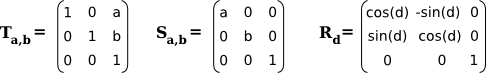
Affine transformations play an essential role in computer graphics, where affine transformations from $\R^3$ to $\R^3$ are represented by $4\times 4$ matrices. In $\R^2$, $3\times 3$ matrices are used. Some of the basic theory in 2D is covered in Section 2.3 of my graphics textbook. Affine transformations in 2D can be built up out of rotations, scaling, and pure translation. These maps are discussed in that section. This illustration from the section shows the $3\times 3$ matrices for the basic transformations:
Things are just a little more complicated in three dimensions, since specifying a rotation in 3D involves specifying an axis of rotation. Often the axis is the x, y, or z axis, but any line in $\R^3$ can be the axis for a rotation. You might take a look at Section 3.5.2 for some very brief information about how matrices are used in 3D graphics.
Section 2.4 explains how composition of affine transformations is used when representing complex objects in computer graphics. An animated demo from that section shows a very simplified 2D scene containing some complex objects that are built up out of simple parts by applying multiple affine transformations. (If you are interested in seeing this animated scene applied as a "texture" on the surfaces of 3D objects, see this demo from Section 4.3.6. Rotate the object by dragging it with your mouse.)
For a completely different application of affine maps, see my chaos game web app. In that program, affine maps are used to create fractals.