Section 7.3
Textures
Most of the WebGL API for working with textures was already covered in Section 6.4. In this section, we look at several examples and techniques for using textures.
7.3.1 Texture Transforms with glMatrix
In Subsection 4.3.4, we saw how to apply a texture transformation in OpenGL. OpenGL maintains a texture transform matrix that can be manipulated to apply scaling, rotation, and translation to texture coordinates before they are used to sample a texture. It is easy to program the same operations in WebGL. We need to compute the texture transform matrix on the JavaScript side. The transform matrix is then sent to a uniform matrix variable in the shader program, where it can be applied to the texture coordinates. Note that as long as the texture transformation is affine, it can be applied in the vertex shader, even though the texture is sampled in the fragment shader. That is, doing the transformation in the vertex shader and interpolating the transformed texture coordinates will give the same result as interpolating the original texture coordinates and applying the transformation to the interpolated coordinates in the fragment shader.
Since we are using glMatrix for coordinate transformation in 3D, it makes sense to use it for texture transforms as well. If we use 2D texture coordinates, we can implement scaling, rotation, and translation on the JavaScript side using the mat3 class from glMatrix. The functions that we need are
- mat3.create() — Returns a new 3-by-3 matrix (represented as an array of length 9). The new matrix is the identity matrix.
- mat3.identity(A) — Sets A to be the identity matrix, where A is an already-existing mat3.
- mat3.translate(A,B,[dx,dy]) — Multiplies the matrix B by a matrix representing translation by (dx,dy), and sets A to be the resulting matrix. A and B must already exist.
- mat3.scale(A,B,[sx,sy]) — Multiplies B by a matrix representing scaling by (sx,sy), and sets A to be the resulting matrix.
- mat3.rotate(A,B,angle) — Multiplies B by a matrix representing rotation by angle radians about the origin, and sets A to be the resulting matrix.
For implementing texture transformations, the parameters A and B in these functions will be the texture transform matrix. For example, to apply a scaling by a factor of 2 to the texture coordinates, we might use the code:
var textureTransform = mat3.create();
mat3.scale( textureTransform, textureTransform, [2,2] );
gl.uniformMatrix3fv( u_textureTransform, false, textureTransform );
The last line assumes that u_textureTransform is the location of a uniform variable of type mat3 in the shader program. (And remember that scaling the texture coordinates by a factor of 2 will shrink the texture on the surfaces to which it is applied.)
The sample WebGL program webgl/texture-transform.html uses texture transformations to animate textures. In the program, texture coordinates are input into the vertex shader as an attribute named a_texCoords of type vec2, and the texture transformation is a uniform variable named textureTransform of type mat3. The transformed texture coordinates are computed in the vertex shader with the GLSL commands
vec3 texcoords = textureTransform * vec3(a_texCoords,1.0);
v_texCoords = texcoords.xy;
Read the source code to see how all this is used in the context of a complete program.
7.3.2 Generated Texture Coordinates
Texture coordinates are typically provided to the shader program as an attribute variable. However, when texture coordinates are not available, it is possible to generate them in the shader program. While the results will not usually look as good as using texture coordinates that are customized for the object that is being rendered, they can be acceptable in some cases.
Generated texture coordinates should usually be computed from the object coordinates of the object that is being rendered. That is, they are computed from the original vertex coordinates, before any transformation has been applied. Then, when the object is transformed, the texture will be transformed along with the object so that it will look like the texture is attached to the object. The texture coordinates could be almost any function of the object coordinates. If an affine function is used, as is usually the case, then the texture coordinates can be computed in the vertex shader. Otherwise, you need to send the object coordinates to the fragment shader in a varying variable and do the computation there.
The simplest idea for generated texture coordinates is simply to use the x and y coordinates from the object coordinate system as the texture coordinates. If the vertex coordinates are given as the value of the attribute variable a_coords, that would mean using a_coords.xy as texture coordinates. This has the effect of projecting the texture onto the surface from the direction of the positive z-axis, perpendicular to the xy-plane. The mapping works OK for a polygon that is facing, more-or-less, in the direction of positive z, but it doesn't give good results for polygons that are edge-on to the xy-plane. Here's what the mapping looks like on a cube:
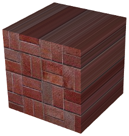
The texture projects nicely onto the front face of the cube. It also works OK on the back face of the cube (not visible in the image), except that it is mirror-reversed. On the other four faces, which are exactly edge-on to the xy-plane, you just get lines of color that come from pixels along the border of the texture image. (In this example, one copy of the texture image exactly fills the front face of the cube. That doesn't happen automatically; you might need a texture transform to adapt the texture image to the surface.)
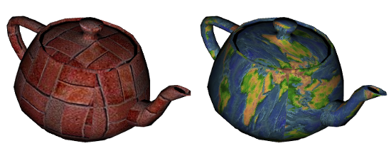
Of course, we could project in other directions to map the texture to other faces of the cube. But how to decide which direction to use? Let's say that we want to project along the direction of one of the coordinate axes. We want to project, approximately at least, from the direction that the surface is facing. The normal vector to the surface tells us that direction. We should project in the direction where the normal vector has its greatest magnitude. For example, if the normal vector is (0.12, 0.85, 0.51), then we should project from the direction of the positive y-axis. And a normal vector equal to (−0.4, 0.56, −0.72) would tell us to project from the direction of the negative z-axis. This resulting "cubical" generated texture coordinates are perfect for a cube, and it looks pretty good on most objects, except that there can be a seam where the direction of projection changes. Here, for example, the technique is applied to a teapot:
When using flat shading, so that all of the normals to a polygon point in the same direction, the computation can be done in the vertex shader. With smooth shading, normals at different vertices of a polygon can point in different directions. If you project texture coordinates from different directions at different vertices and interpolate the results, the result is likely to be a mess. So, doing the computation in the fragment shader is safer. Suppose that the interpolated normal vectors and object coordinates are provided to the fragment shader in varying variables named v_normal and v_objCoords. Then the following code can be used to generate "cubical" texture coordinates:
if ( (abs(v_normal.x) > abs(v_normal.y)) &&
                                (abs(v_normal.x) > abs(v_normal.z)) ) {
    // project along the x-axis
    texcoords = (v_normal.x > 0.0) ? v_objCoords.yz : v_objCoords.zy;
}
else if ( (abs(v_normal.z) > abs(v_normal.x)) &&
                                (abs(v_normal.z) > abs(v_normal.y)) ) {
    // project along the z-axis
    texcoords = (v_normal.z > 0.0) ? v_objCoords.xy : v_objCoords.yx;
}
else {
    // project along the y-axis
    texcoords = (v_normal.y > 0.0) ? v_objCoords.zx : v_objCoords.xz;
}
When projecting along the x-axis, for example, the y and z coordinates from v_objCoords are used as texture coordinates. The coordinates are computed as either v_objCoords.yz or v_objCoords.zy, depending on whether the projection is from the positive or the negative direction of x. The order of the two coordinates is chosen so that a texture image will be projected directly onto the surface, rather than mirror-reversed.
You can experiment with generated textures using the following demo. The demo shows a variety of textures and objects using cubical generated texture coordinates, as discussed above. You can also try texture coordinates projected just onto the xy or zx plane, as well as a cylindrical projection that wraps a texture image once around a cylinder. A final option is to use the x and y coordinates from the eye coordinate system as texture coordinates. That option fixes the texture on the screen rather than on the object, so the texture doesn't rotate with the object. The effect is interesting, but probably not very useful.
7.3.3 Procedural Textures
Up until now, all of our textures have been image textures. With an image texture, a color is computed by sampling the image, based on a pair of texture coordinates. The image essentially defines a function that takes texture coordinates as input and returns a color as output. However, there are other ways to define such functions besides looking up values in an image. A procedural texture is defined by a function whose value is computed rather than looked up. That is, the texture coordinates are used as input to a code segment whose output is the corresponding color value for the texture.
In WebGL, procedural textures can be defined in the fragment shader. The idea is simple: Take a vec2 representing a set of texture coordinates. Then, instead of using a sampler2D to look up a color, use the vec2 as input to some mathematical computation that computes a vec4 representing a color. In theory any computation could be used, as long as the components of the vec4 are in the range 0.0 to 1.0.
We can even extend the idea to 3D textures. 2D textures use a vec2 as texture coordinates. For 3D texture coordinates, we use a vec3. Instead of mapping points on a plane to color, a 3D texture maps points in space to colors. It's possible to have 3D textures that are similar to image textures. That is, a color value is stored for each point in a 3D grid, and the texture is sampled by looking up colors in the grid. However, a 3D grid of colors takes up a lot of memory. On the other hand, 3D procedural textures use no memory resources and use very little more computational resources than 2D procedural textures.
So, what can be done with procedural textures? In fact, quite a lot. There is a large body of theory and practice related to procedural textures. We will look at a few of the possibilities. Here's a torus, textured using four different procedural textures. The images are from the demo shown at the end of this subsection:
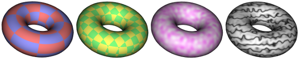
The torus on the left uses a 2D procedural texture representing a checkerboard pattern. The 2D texture coordinates were provided, as usual, as values of a vertex attribute variable in the shader program. The checkerboard pattern is regular grid of equal-sized colored squares, but, as with any 2D texture, the pattern is stretched and distorted when it is mapped to the curved surface of the torus. Given texture coordinates in the varying variable v_texCoords, the color value for the checkerboard texture can be computed as follows in the fragment shader:
vec4 color;
float a = floor(v_texCoords.x * scale);
float b = floor(v_texCoords.y * scale);
if (mod(a+b, 2.0) > 0.5) {  // a+b is odd
    color = vec3(1.0, 0.5, 0.5, 1.0); // pink
}
else {  // a+b is even
    color = vec3(0.6, 0.6, 1.0, 1.0); // light blue
}
The scale in the second and third lines represents a texture transformation that is used to adapt the size of the texture to the object that is being textured. (The texture coordinates for the torus range from 0 to 1; without the scaling, only one square in the checkerboard pattern would be mapped to the torus. For the torus in the picture, scale is 8.) The floor function computes the largest integer less than or equal to its parameter, so a and b are integers. The value of mod(a+b,2.0) is either 0.0 or 1.0, so the test in the fourth line tests whether a+b is even or odd. The idea here is that when either a or b increases or decreases by 1, a+b will change from even to odd or from odd to even; that ensures that neighboring squares in the pattern will be differently colored.
The second torus in the illustration uses a 3D checkerboard pattern. The 3D pattern is made up of a grid of cubes that alternate in color in all three directions. For the 3D texture coordinates on the cube, I use object coordinates. That is, the 3D texture coordinates for a point are the same as its position in space, in the object coordinate system in which the torus is defined. The effect is like carving the torus out of a solid block that is colored, inside and out, with a 3D checkerboard pattern. Note that you don't see colored squares or rectangles on the surface of the torus; you see the intersections of that surface with colored cubes. The intersections have a wide variety of shapes. That might be a disadvantage for this particular 3D texture, but the advantage is that there is no stretching and distortion of the texture. The code for computing the 3D checkerboard is the same as for the 2D case, but using three object coordinates instead of two texture coordinates.
Natural-looking textures often have some element of randomness. We can't use actual randomness, since then the texture would look different every time it is drawn. However, some sort of pseudo-randomness can be incorporated into the algorithm that computes a texture. But we don't want the colors in the texture to look completely random—there has to be some sort of pattern in the pattern! Many natural-looking procedural textures are based on a type of pseudo-randomness called Perlin noise, named after Ken Perlin who invented the algorithm in 1983. The third torus in the above illustration uses a 3D texture based directly on Perlin noise. The "marble" texture on the fourth torus uses Perlin noise as a component in the computation. Both textures are 3D, but similar 2D versions are also possible. (I don't know the algorithm for Perlin noise. I copied the GLSL code from https://github.com/ashima/webgl-noise. The code is published under an MIT-style open source license, so that it can be used freely in any project.)
In the sample program, 3D Perlin noise is computed by a function snoise(v), where v is a vec3 and the output of the function is a float in the range −1.0 to 1.0. Here is the computation:
float value = snoise( scale*v_objCoords );
value = 0.75 + value*0.25; // map to the range 0.5 to 1.0
color = vec3(1.0,value,1.0);
Here, v_objCoords is a varying variable containing the 3D object coordinates of the point that is being textured, and scale is a texture transformation that adapts the size of the texture to the torus. Since the output of snoise() varies between −1.0 and 1.0, value varies from 0.5 to 1.0, and the color for the texture ranges from pale magenta to white. The color variation that you see on the third torus is characteristic of Perlin noise. The pattern is somewhat random, but it has regular, similarly sized features. With the right scaling and coloration, basic Perlin noise can make a decent cloud texture.
The marble texture on the fourth torus in the illustration is made by adding some noise to a regular, periodic pattern. The basic technique can produce a wide variety of useful textures. The starting point is a periodic function of one variable, with values between 0.0 and 1.0. To get a periodic pattern in 2D or 3D, the input to the function can be computed from the texture coordinates. Different functions can produce very different effects. The three patterns shown here use the functions (1.0+sin(t))/2.0, abs(sin(t)) and (t−floor(t)), respectively:
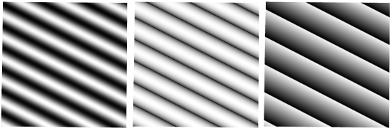
In the second image, taking the absolute value of sin(t) produces narrower, sharper dark bands than the plain sine function in the first image. This is the function that is used for the marble texture in the illustration. The sharp discontinuity in the third image can be an interesting visual effect.
To get the 2D pattern from a function f(t) of one variable, we can use a function of a vec2, v, defined as f(a*v.x+b*v.y), where a and b are constants. The values of a and b determine the orientation and spacing of the color bands in the pattern. For a 3D pattern, we would use f(a*v.x+b*v.y+c*v.z).
To add noise to the pattern, add a Perlin noise function to the input of the function. For a 3D pattern, the function would become
f( a*v.x + b*v.y + c*v.z + d*snoise(e*v) )
The new constants d and e determine the size and intensity of the perturbations to the pattern. As an example, the code that creates the marble texture for the torus is:
vec3 v = v_objCoords*scale;
float t = (v.x + 2.0*v.y + 3.0*v.z);
t += 1.5*snoise(v);
float value =  abs(sin(t));
color = vec3(sqrt(value));
(The sqrt at the end was added to make the color bands even sharper than they would be without it.)
The following demo lets you apply a variety of 3D textures to different objects. The procedural textures used in the demo are just a small sample of the possibilities.
7.3.4 Bumpmaps
So far, the only textures that we have encountered have affected color. Whether they were image textures, environment maps, or procedural textures, their effect has been to vary the color on the surfaces to which they were applied. But, more generally, texture can refer to variation in any property. One example is bumpmapping, where the property that is modified by the texture is the normal vector to the surface. A normal vector determines how light is reflected by the surface, which is a major visual clue to the direction that the surface faces. Modifying the normal vectors has the effect of modifying the apparent orientation of the surface, as least with respect to the way it reflects light. It can add the appearance of roughness or "bumps" to the surface. The effect can be visually similar to changing the positions of points on the surface, but with bumpmapping the change in appearance is achieved without actually changing the surface geometry. The alternative approach of modifying the actual geometry, which is called "displacement mapping," can give better results but requires a lot more computational and memory resources.
The typical way to do bumpmapping is with a height map. A height map, is a grayscale image in which the variation in color is used to specify the amount by which points on the surface are (or appear to be) displaced. A height map is mapped to a surface in the same way as an image texture, using texture coordinates that are supplied as an attribute variable or generated computationally. But instead of being used to modify the color of a pixel, the color value from the height map is used to modify the normal vector that goes into the lighting equation that computes the color of the pixel. A height map that is used in this way is also called a bump map. I'm not sure that my implementation of this idea is optimal, but it can produce pretty good results.
Here are two examples. For each example, a bumpmapped torus is shown next to the height map that was applied to the torus:
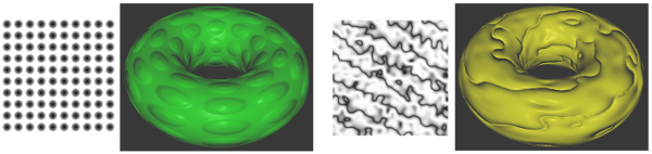
In the first example, the gray dots in the height map produce the appearance of bumps on the torus. The darker the color from the map, the greater apparent displacement of the point on the surface. The black centers of the dots map to the tops of the bumps. For the second example, the dark curves in the height map seem to produce deep grooves in the surface. As is usual for textures, the height maps have been stretched to cover the torus, which distorts the shape of the features from the map.
To see how bumpmapping can be implemented, let's first imagine that we want to apply it to a one-dimensional "surface." Consider a normal vector to a point on the surface, and suppose that a height map texture is applied to the surface. Take a vector, shown in black in the following illustration, that points in the direction in which the height map grayscale value is decreasing.
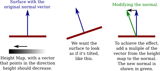
We want the surface to appear as if it is tilted, as shown in the middle of the illustration. (I'm assuming here that darker colors in the height map correspond to smaller heights.) Literally tilting the surface would change the direction of the normal vector. We can get the same change in the normal vector by adding some multiple of the vector from the height map to the original normal vector, as shown on the right above. Changing the number that is multiplied by the height map vector changes the degree of tilting of the surface. Increasing the multiplier gives a stronger bump effect. Using a negative multiple will tilt the surface in the opposite direction, which will transform "bumps" into "dimples," and vice versa. I will refer to the multiplier as the bump strength.
Things get a lot more complicated for two-dimensional surfaces in 3D space. A 1D "surface" can only be tilted left or right. On a 2D surface, there are infinitely many directions to tilt the surface. Note that the vector that points in the direction of tilt points along the surface, not perpendicular to the surface. A vector that points along a surface is called a tangent vector to the surface. To do bump mapping, we need a tangent vector for each point on the surface. Tangent vectors will have to be provided, along with normal vectors, as part of the data for the surface. For my version of bumpmapping, the tangent vector that we need should be coordinated with the texture coordinates for the surface: The tangent vector should point in the direction in which the s coordinate in the texture coordinates is increasing.
In fact, to properly account for variation in the height map, we need a second tangent vector. The second tangent vector is perpendicular both to the normal and to the first tangent vector. It is commonly called the "binormal" vector, and it can be computed from the normal and the tangent. (The binormal should point in the direction in which the t texture coordinate is increasing, but whether that can be exactly true will depend on the texture mapping. As long as it's not too far off, the result should be OK.)
Now, to modify the normal vector, proceed as follows: Sample the height maps at two points, separated by a small difference in the s coordinate. Let a be the difference between the two values; a represents the rate at which the height value is changing in the direction of the tangent vector (which, remember, points in the s direction along the surface). Then sample the height map at two points separated by a small difference in the t coordinate, and let b be the difference between the two values, so that b represents the rate at which the height value is changing in the direction of the binormal vector. Let D be the vector a*T + b*B, where T is the tangent vector and B is the binormal. Then add D, or a multiple of D, to the original normal vector to produce the modified normal that will be used in the lighting equation. (If you know multivariable calculus, what we are doing here amounts to using approximations for directional derivatives and the gradient vector of a height function on the surface.)
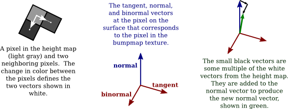
I have tried to explain the procedure in the following illustration. You need to visualize the situation in 3D, noting that the normal, tangent, and binormal vectors are perpendicular to each other. The white arrows on the left are actually multiples of the binormal and tangent vectors, with lengths given by the change in color between two pixels.
The sample program webgl/bumpmap.html demonstrates bumpmapping. The two bumpmapped toruses in the above illustration are from that program. When you run the program, pay attention to the specular highlights! They will help you to see how a bumpmap texture differs from an image texture. The effect might be more obvious if you change the "Diffuse Color" from white to some other color. The specular color is always white.
(For this program, I had to add tangent vectors to my objects. I chose three objects—a cube, a cylinder, and a torus—for which tangent vectors were relatively easy to compute. But, honestly, it took me a while to get all the tangent vectors pointing in the correct directions.)
The bumpmapping is implemented in the fragment shader in the sample program. The essential problem is how to modify the normal vector. Let's examine the GLSL code that does the work:
vec3 normal = normalize( v_normal );
vec3 tangent = normalize( v_tangent );
vec3 binormal = cross(normal,tangent);

float bm0, bmUp, bmRight;  // Samples from the bumpmap at three texels.
bm0 = texture2D( bumpmap, v_texCoords ).r;
bmUp = texture2D( bumpmap, v_texCoords + vec2(0.0, 1.0/bumpmapSize.y) ).r;
bmRight = texture2D( bumpmap, v_texCoords + vec2(1.0/bumpmapSize.x, 0.0) ).r;

vec3 bumpVector = (bmRight - bm0)*tangent + (bmUp - bm0)*binormal;
normal += bumpmapStrength*bumpVector;
normal = normalize( normalMatrix*normal );
The first three lines compute the normal, tangent, and binormal unit vectors. The normal and tangent come from varying variables whose values are interpolated from attribute variables, which were in turn input to the shader program from the JavaScript side. The binormal, which is perpendicular to both the normal and the tangent, is computed as the cross product of the normal and tangent (Subsection 3.5.1).
The next four lines get the values of the height map at the pixel that corresponds to the surface point that is being processed and at two neighboring pixels. bm0 is the height map value at the current pixel, whose coordinates in the texture are given by the texture coordinates, v_texCoords. The value for bm0 is the red color component from the bumpmap texture; since the texture is grayscale, all of its color components have the same value. bmUp is the value from the pixel above the current pixel in the texture; the coordinates are computed by adding 1.0/bumpmapSize.y to the y-coordinate of the current pixel, where bumpmapSize is a uniform variable that gives the size of the texture image, in pixels. Since texture coordinates in the image run from 0.0 to 1.0, the difference in the y-coordinates of the two pixels is 1.0/bumpmapSize.y. Similarly, bmRight is the height map value for the pixel to the right of the current pixel in the bumpmap texture. I should note that the minification filter for the bumpmap texture was set to gl.NEAREST, because we need to read the actual value from the texture, not a value averaged from several pixels, as would be returned by the default minification filter.
The two vectors (bmRight−bm0)*tangent and (bmUp−bm0)*binormal are the two white vectors in the above illustration. Their sum is bumpVector. A multiple of that sum is added to the normal vector to give the modified normal vector. The multiplier, bumpmapStrength, is a uniform float variable.
All of the calculations so far have been done in the object coordinate system. The resulting normal depends only on the original object coordinates, not on any transformation that has been applied. The normal vector still has to be transformed into eye coordinates before it can be used in the lighting equation. That transformation is done in the last line of code shown above.
7.3.5 Environment Mapping
Subsection 5.3.5 showed how to use environment mapping in three.js to make it look like the surface of an object reflects an environment. Environment mapping uses a cubemap texture, and it is really just a way of mapping a cubemap texture to the surface. It doesn't make the object reflect other objects in its environment. We can make it look as if the object is reflecting its environment by adding a skybox—a large cube surrounding the scene, with the cubemap mapped onto its interior. However, the object will only seem to be reflecting the skybox. And if there are other objects in the environment, they won't be part of the reflection.
The sample program webgl/skybox-and-env-map.html implements environment mapping in WebGL. The program shows a single fully reflective object inside a skybox. No lighting is used in the scene; the colors for both the skybox and the object are taken directly from the cubemap texture. The object looks like a perfect mirror. This is not the only way of using an environment map. For example, a basic object color could be computed using the lighting equation—perhaps even with an image texture—and the environment map could be blended with the basic color to give the appearance of a shiny but not fully reflective surface. However, the point of the sample program is just to show how to use a skybox and environment map in WebGL. The shader programs that are used to do that are actually quite short.
As for the cubemap texture itself, Subsection 6.4.4 showed how to load a cubemap texture as six separate images and how to access that texture in GLSL using a variable of type samplerCube. Remember that a cubemap texture is sampled using a 3D vector that points from the origin towards the point on the cube where the texture is to be sampled.
It's easy to render the skybox: Draw a large cube, centered at the origin, enclosing the scene and the camera position. To color a pixel in the fragment shader, sample the cubemap texture using a vector that points from the origin through the point on the cube that is being rendered, so that the color of a point on the cube is the same as the color of the corresponding point in the cubemap. Note that it is the cube's object coordinates that are used to sample the texture, since the texture should be attached to the cube when we rotate the view.
In the shader program for rendering a skybox, the vertex shader just needs to compute gl_Position as usual and pass the object coordinates on to the fragment shader in a varying variable. Here is the vertex shader source code for the skybox:
uniform mat4 projection;
uniform mat4 modelview;
attribute vec3 coords;
varying vec3 v_objCoords;
void main() {
    vec4 eyeCoords = modelview * vec4(coords,1.0);
    gl_Position = projection * eyeCoords;
    v_objCoords = coords;
}
And the fragment shader simply uses the object coordinates to get the fragment color by sampling the cubemap texture:
precision mediump float;
varying vec3 v_objCoords;
uniform samplerCube skybox;
void main() {
      gl_FragColor = textureCube(skybox, v_objCoords);
}
Note that the vector that is used to sample a cubemap texture does not have to be a unit vector; it just has to point in the correct direction.
To understand how a cube map texture can be applied to an object as a reflection map, we have to ask what point from the texture should be visible at a point on the object? If we think of the texture as an actual environment, then a ray of light would come from the environment, hit the object, and be reflected towards the viewer. We just have to trace that light ray back from the viewer to the object and then to the environment. The direction in which the light ray is reflected is determined, as always, by the normal vector. Consider a 2D version of the geometry. You can think of this as a cross-section of the 3D geometry:
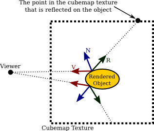
In this illustration, the dotted box represents the cubemap texture. (You really should think of it as being at infinite distance.) V is a vector that points from the object towards the viewer. N is the normal vector to the surface. And R is the reflection of V through N. R points to the texel in the cubemap texture that is visible to the viewer at the point on the surface; it is the vector that is needed to sample the cubemap texture. The picture shows the three vectors at two different points on the surface. In GLSL, R can be computed as −reflect(V, N).
If the same cubemap texture is also applied to a skybox, it will look as if the object is reflecting the skybox—but only if no transformation has been applied to the skybox cube. The reason is that transforming the skybox does not automatically transform the cubemap texture. Since we want to be able to rotate the view, we need to be able to transform the skybox. And we want the reflected object to look like it is reflecting the skybox in its transformed position, not in its original position. That viewing transformation can be thought of as a modeling transformation on the skybox, as well as on other objects in the scene. We have to figure out how to make it apply to the cubemap texture. Let's think about what happens in the 2D case when we rotate the view by −30 degrees. That's the same as rotating the skybox and object by 30 degrees. In the illustration, I've drawn the viewer at the same position as before, and I have rotated the scene. The square with the fainter dotted outline is the skybox. The cubemap texture hasn't moved:
![]()
If we compute R as before and use it to sample the cubemap texture, we get the wrong point in the texture. The viewer should see the point where R intersects the skybox, not the point where R intersects the texture. The correct point in the texture is picked out by the vector T. T is computed by transforming R by the inverse of the viewing transformation. R was rotated by the viewing transformation; the inverse viewing transformation undoes that transformation, putting T into the same coordinate system as the cube map. In this case, since R was rotated by 30 degrees, a rotation of −30 degrees is applied to compute T. (This is just one way to understand the geometry. If you prefer to think of the cubemap as rotating along with the skybox, then we need to apply a texture transformation to the texture—which is another way of saying that we need to transform R before using it to sample the texture.)
In the sample program, the shader program that is used to represent the object is different from the one used to render the skybox. The vertex shader is very typical. Note that the modelview transformation can include modeling transforms that are applied to the object in addition to the viewing transform that is applied to the entire scene. Here is the source code:
uniform mat4 projection;
uniform mat4 modelview;
attribute vec3 coords;
attribute vec3 normal;
varying vec3 v_eyeCoords;
varying vec3 v_normal;
void main() {
    vec4 eyeCoords = modelview * vec4(coords,1.0);
    gl_Position = projection * eyeCoords;
    v_eyeCoords = eyeCoords.xyz;
    v_normal = normalize(normal);
}
The vertex shader passes eye coordinates to the fragment shader in a varying variable. In eye coordinates, the viewer is at the point (0,0,0), and the vector V that points from the surface to the viewer is simply −v_eyeCoords.
The source code for the fragment shader implements the algorithm discussed above for sampling the cubemap texture. Since we are doing perfect reflection, the color for the fragment comes directly from the texture:
precision mediump float;
varying vec3 vCoords;
varying vec3 v_normal;
varying vec3 v_eyeCoords;
uniform samplerCube skybox;
uniform mat3 normalMatrix;
uniform mat3 inverseViewTransform;
void main() {
      vec3 N = normalize(normalMatrix * v_normal);
      vec3 V = -v_eyeCoords;
      vec3 R = -reflect(V,N);
      vec3 T = inverseViewTransform * R;
      gl_FragColor = textureCube(skybox, T);
}
The inverseViewTransform is computed on the JavaScript side from the modelview matrix, after the viewing transform has been applied but before any addition modeling transformation is applied, using the commands
mat3.fromMat4(inverseViewTransform, modelview);
mat3.invert(inverseViewTransform,inverseViewTransform);
We need a mat3 to transform a vector. The first line discards the translation part of the modelview matrix, putting the result in inverseViewTransform. Translation doesn't affect vectors, but the translation part is zero in any case since the viewing transformation in this program is just a rotation. The second line converts inverseViewTransform into its inverse.